Understanding Macros and VBA in Excel
Macros are like your best friends in Excel. They automate repetitive tasks and save you copious amounts of time—something we all could use more of, right? For instance, if you find yourself regularly generating financial reports every month, imagine not having to click through all those menus! Instead, just press a button and let Excel do the heavy lifting.
Visual Basic for Applications (VBA) is the programming language behind macros. It may sound intimidating, but trust me, once you get the hang of it, you’ll wonder how you ever lived without it. In Excel 365, for instance, recording a macro is just a few clicks away. In this guide, we’ll walk through the process step-by-step, making it accessible to beginners like you!

Why Use Macros?
- Streamline Processes: Imagine spending half an hour formatting a sales report only to find out that you missed a cell. With macros, it’s click-and-go!
- Consistency: Macros ensure that your tasks are performed the same way every time. No more worrying whether you remembered all the steps.
- Time-Saving: Why do the same task repeatedly when you can record it once? Think about it—instead of manually updating your inventory spreadsheet with sales data each week, just run a macro to pull and format the data for you.
Recording Your First Macro in Excel
Ready for your first taste of macro magic? Here’s how to record one in Excel 2021. The steps are pretty much the same across different versions, but you might notice some placement differences.
- Open your Excel workbook.
- Go to the View tab on the Ribbon.
- Click on Macros and then Record Macro.
- Give your macro a name—no spaces allowed! I usually go for something descriptive, like
FormatSalesReport. - Assign it a shortcut key (for example,
Ctrl+Shift+R) for quick access. Just remember to choose a combination that doesn’t clash with existing shortcuts. - Hit OK to start recording your actions.
Now go ahead and perform the tasks you want to automate—formatting data, entering formulas, whatever you need! Once you’re done, go back to the View tab, click on Macros, and then select Stop Recording.
Editing Your Macro with VBA
So, you've recorded a macro, and now you're feeling like a rock star. But wait—what if you want to tweak it? This is where VBA comes into play. Let’s roll up our sleeves and dive into some code.
- Press
Alt + F11to open the VBA editor. - On the left sidebar, find your macro under “Modules.” It should look something like
Module1. - Double-click on it, and a window will pop up showing your recorded macro code.
Now, if you want to make it even snazzier, you can add loops, conditionals, and other commands. For example, if your report needs to highlight sales that are below a certain threshold, you could incorporate an If statement to do just that.
Common Mistakes when Working with Macros
Na minha experiência, even seasoned users make a few mistakes with macros. Here’s a list of the most notorious ones to avoid:
- Not Saving Your Workbook as Macro-Enabled: If you don't save your file as
.xlsm, your macro will be lost! Excel will save it like any regular workbook, and that would be a bummer. - Over-recording: Sometimes, people get a bit too ambitious and record every little action. This can result in a messy, bloated macro that’s hard to maintain. Keep it neat!
- Hardcoding Values: Avoid putting fixed values directly into your macros. If you need to change something, it’s a pain to dig through the code. Instead, use cell references or input boxes.
Practical Applications of Macros
Let’s get down to the nitty-gritty—how can you use macros in your day-to-day activities? Here are some real-world examples:
- Financial Reporting: Automate formatting, calculations, and compiling data from different sheets. For example, if your monthly financial report consists of data from five sheets, record a macro that pulls, formats, and presents the data in one summary sheet.
- Sales Tracking: Update sales records automatically. This could mean applying specific filters to identify top-performing salespeople or products. You could even create a button on your dashboard that runs a macro to refresh your sales data with a single click!
- HR Onboarding: New employee data entry often requires repetitive tasks like filling out forms. Use a macro to auto-fill standard information or create reports based on new hires.
Dica DomineTec: Always test your macros on a copy of your file first to avoid losing any important data!

Exploring the Power of Excel 365 and Excel 2021
If you have ever found yourself staring at a massive financial dataset in Excel 365, you know how crucial the right tools can be. Many functions often live in the shadow of VLOOKUP, but their utility is unquestionable when dealing with reports where months or weeks are laid out in contiguous columns. Unlike older versions such as Excel 2019, recent releases bring an upgraded calculation engine that makes processing giant spreadsheets much faster, avoiding those dreaded crashes (we've all furiously hit Ctrl+S praying Excel doesn't close on us!).
The secret to mastering this is understanding how your data structure dictates performance. Imagine a retail sales dashboard: products are listed in rows, but the January-to-December results are spread across columns. Using the proper syntax allows you to instantly locate a specific month's revenue. By locking the array with the F4 key, you ensure that when you drag the formula down (or simply use Ctrl+C and Ctrl+V), the reference stays static, avoiding the classic #N/A error.
It is worth noting that while Excel Online is fantastic for collaboration, massive volumes of data searched via arrays might experience a slight delay during cloud recalculations. Still, for inventory management and dynamic HR dashboards, these functions remain a pillar of workplace productivity. And if you think you are limited to the basics, try combining features with the MATCH function to create dynamic row indices. This transforms a rigid spreadsheet into an intelligent query system worthy of a senior analyst.
Advanced Tips: Avoiding Common Errors and Optimizing Performance
Nobody likes opening a spreadsheet to find a sea of #N/A or #VALUE! errors. When this happens, panic might set in, but the solution is usually straightforward. One of the biggest culprits behind formula failures is invisible text formatting. You know that trailing whitespace that sneaks in when you export data from the company's ERP system? It prevents Excel from recognizing your search criteria. The golden tip here is to nest the TRIM function inside your formulas: =VLOOKUP(TRIM(A2), Array, 2, FALSE). This cleans the invisible garbage out of your data before the search even begins.
Another classic scenario happens in P&L (Profit and Loss) reports where new rows are constantly inserted. If you hardcoded the row index number in your formula (e.g., row 5), adding a new category above it means your spreadsheet will return the wrong value, as the desired row is now row 6. An elegant workaround is using the ROW() function combined, or better yet, formatting your data as a Table (shortcut Ctrl+T). Excel tables name ranges automatically, meaning your arrays dynamically scale with your data growth seamlessly.
Whether you are on Mac or Windows, the principle remains the same. In Excel for Mac, shortcuts like Command+C replace Ctrl+C, but the syntactical logic is entirely intact. I often joke that Excel is a universal language: once you grasp the fluency of arrays and absolute vs. relative referencing, the operating system is just a minor detail. Diving deep into the nuances of Excel is an investment that saves countless hours of manual, mind-numbing "copy and paste" work.
Integrating with Dashboard and Visualization Tools
When we start building visual dashboards, the accuracy of data extraction is paramount. This is where Excel joins forces with other tools to create flawless control panels. One of the smartest ways to deploy this logic is by tying it to dropdown menus (Data Validation). By allowing a user to select, say, the "Quarter" from a dropdown list, Excel works behind the scenes to fetch the exact column for that quarter and feed the primary chart.
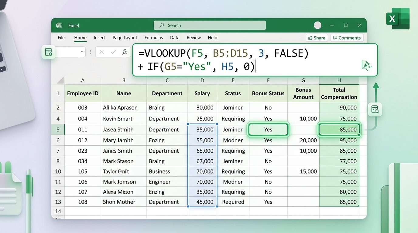
Think about the daily grind of an HR department. Every month, they must compile overtime, time banks, and absences for dozens of employees. If the system generates horizontally oriented reports (days of the month across columns), it is the ideal conduit to extract specific info into an individual employee's file. If you make a mistake during the setup, a quick Ctrl+Z undoes the mess in a second, but a well-constructed layout greatly minimizes the need for manual intervention.
There is even more: when dealing with complex reports in Excel 365, you can also explore integrating your table with Power Query. Keep your data clean at the source, and use Excel simply as a display bridge. Remember, the secret to productivity isn't always using the most complex function out there; it is about using the right tool for the data structure you have. If your database grows horizontally (columns added over time), do not force a rigid layout. Accept the nature of your data and let the software do the heavy lifting for you.
Real-World Use Cases: Inventory and Sales Management
For those working in retail or e-commerce, inventory control can quickly become a logistical nightmare. Suppose you receive weekly price updates from suppliers, and these prices are delivered in spreadsheets where columns represent the weeks of the year. How do you efficiently update your cost base? The answer, once again, lies in the strategic use of native features.
By defining a robust structure, you can build a "Current Cost" table that always pulls the value from the latest registered week. This can be achieved by pairing lookups with functions that count non-empty cells (COUNTA). So, if you are currently in Week 42, the formula automatically locates that column and retrieves the product's value from the corresponding row. This level of automation eliminates manual typing, which is historically the primary cause of pricing errors.
Such practices are widely adopted by companies that demand agility in decision-making. I have seen many chaotic operational processes brought to order simply by introducing a solid reporting structure. The sheer flexibility of Excel 2021 and Microsoft 365 to rapidly recalculate dynamic arrays means that even 50,000-row, 100-column spreadsheets can run without lag—provided you avoid referencing entire infinite columns unnecessarily. Keep your data confined to the actual data boundaries to ensure top-tier performance.
Exploring the Power of Excel 365 and Excel 2021
If you have ever found yourself staring at a massive financial dataset in Excel 365, you know how crucial the right tools can be. Many functions often live in the shadow of VLOOKUP, but their utility is unquestionable when dealing with reports where months or weeks are laid out in contiguous columns. Unlike older versions such as Excel 2019, recent releases bring an upgraded calculation engine that makes processing giant spreadsheets much faster, avoiding those dreaded crashes (we've all furiously hit Ctrl+S praying Excel doesn't close on us!).
The secret to mastering this is understanding how your data structure dictates performance. Imagine a retail sales dashboard: products are listed in rows, but the January-to-December results are spread across columns. Using the proper syntax allows you to instantly locate a specific month's revenue. By locking the array with the F4 key, you ensure that when you drag the formula down (or simply use Ctrl+C and Ctrl+V), the reference stays static, avoiding the classic #N/A error.
It is worth noting that while Excel Online is fantastic for collaboration, massive volumes of data searched via arrays might experience a slight delay during cloud recalculations. Still, for inventory management and dynamic HR dashboards, these functions remain a pillar of workplace productivity. And if you think you are limited to the basics, try combining features with the MATCH function to create dynamic row indices. This transforms a rigid spreadsheet into an intelligent query system worthy of a senior analyst.
Advanced Tips: Avoiding Common Errors and Optimizing Performance
Nobody likes opening a spreadsheet to find a sea of #N/A or #VALUE! errors. When this happens, panic might set in, but the solution is usually straightforward. One of the biggest culprits behind formula failures is invisible text formatting. You know that trailing whitespace that sneaks in when you export data from the company's ERP system? It prevents Excel from recognizing your search criteria. The golden tip here is to nest the TRIM function inside your formulas: =VLOOKUP(TRIM(A2), Array, 2, FALSE). This cleans the invisible garbage out of your data before the search even begins.
Another classic scenario happens in P&L (Profit and Loss) reports where new rows are constantly inserted. If you hardcoded the row index number in your formula (e.g., row 5), adding a new category above it means your spreadsheet will return the wrong value, as the desired row is now row 6. An elegant workaround is using the ROW() function combined, or better yet, formatting your data as a Table (shortcut Ctrl+T). Excel tables name ranges automatically, meaning your arrays dynamically scale with your data growth seamlessly.
Whether you are on Mac or Windows, the principle remains the same. In Excel for Mac, shortcuts like Command+C replace Ctrl+C, but the syntactical logic is entirely intact. I often joke that Excel is a universal language: once you grasp the fluency of arrays and absolute vs. relative referencing, the operating system is just a minor detail. Diving deep into the nuances of Excel is an investment that saves countless hours of manual, mind-numbing "copy and paste" work.
Integrating with Dashboard and Visualization Tools
When we start building visual dashboards, the accuracy of data extraction is paramount. This is where Excel joins forces with other tools to create flawless control panels. One of the smartest ways to deploy this logic is by tying it to dropdown menus (Data Validation). By allowing a user to select, say, the "Quarter" from a dropdown list, Excel works behind the scenes to fetch the exact column for that quarter and feed the primary chart.
Think about the daily grind of an HR department. Every month, they must compile overtime, time banks, and absences for dozens of employees. If the system generates horizontally oriented reports (days of the month across columns), it is the ideal conduit to extract specific info into an individual employee's file. If you make a mistake during the setup, a quick Ctrl+Z undoes the mess in a second, but a well-constructed layout greatly minimizes the need for manual intervention.
There is even more: when dealing with complex reports in Excel 365, you can also explore integrating your table with Power Query. Keep your data clean at the source, and use Excel simply as a display bridge. Remember, the secret to productivity isn't always using the most complex function out there; it is about using the right tool for the data structure you have. If your database grows horizontally (columns added over time), do not force a rigid layout. Accept the nature of your data and let the software do the heavy lifting for you.
Real-World Use Cases: Inventory and Sales Management
For those working in retail or e-commerce, inventory control can quickly become a logistical nightmare. Suppose you receive weekly price updates from suppliers, and these prices are delivered in spreadsheets where columns represent the weeks of the year. How do you efficiently update your cost base? The answer, once again, lies in the strategic use of native features.
By defining a robust structure, you can build a "Current Cost" table that always pulls the value from the latest registered week. This can be achieved by pairing lookups with functions that count non-empty cells (COUNTA). So, if you are currently in Week 42, the formula automatically locates that column and retrieves the product's value from the corresponding row. This level of automation eliminates manual typing, which is historically the primary cause of pricing errors.
Such practices are widely adopted by companies that demand agility in decision-making. I have seen many chaotic operational processes brought to order simply by introducing a solid reporting structure. The sheer flexibility of Excel 2021 and Microsoft 365 to rapidly recalculate dynamic arrays means that even 50,000-row, 100-column spreadsheets can run without lag—provided you avoid referencing entire infinite columns unnecessarily. Keep your data confined to the actual data boundaries to ensure top-tier performance.
Frequently Asked Questions
What versions of Excel support macros?
Macros are supported in Excel 2010 and later, including Excel 2013, Excel 2016, Excel 2019, Excel 2021, and Excel 365, as well as Excel for Mac. Just make sure to save your workbooks as .xlsm for your macros to be saved.
Can I create a macro without knowing VBA?
Absolutely! You can record macros without writing any VBA code at all. However, learning some basic VBA will allow for more advanced customizations and better control over your macros.
Is there a way to share my macros with others?
Yes, you can share your macro-enabled workbooks (.xlsm files) with others. If someone else needs to use your macros, they’ll also need to enable macros in their settings when they open your file.
Can I run macros in Excel Online?
Unfortunately, macros do not work in Excel Online. You’ll need to use a desktop version of Excel for running and recording macros.
How can I troubleshoot if my macro isn’t working?
Check for common errors such as unrecognized commands, incorrect references, or forgotten steps. The debugger in the VBA editor is your friend! You can step through your code to find where things are going awry.