
Understanding VLOOKUP: The Basics
When it comes to Excel, the VLOOKUP function is often touted as a lifesaver. Imagine you're an HR manager, and you need to pull employee salaries from a massive spreadsheet containing various details. Instead of manually sorting through rows of data, you can use VLOOKUP to find what you need in seconds. Trust me, it’s as glorious as it sounds!
Let’s break it down. VLOOKUP stands for "Vertical Lookup," and it's primarily used to search for a value in the first column of a table and return a value in the same row from a specified column. Let’s say you have a table of products with their prices. You can look up a product name and fetch its price without lifting a finger—well, almost!
The VLOOKUP Formula Explained
The syntax for VLOOKUP isn’t as intimidating as it looks, I promise. It goes like this:
=VLOOKUP(lookup_value, table_array, col_index_num, [range_lookup])
- lookup_value: This is the value you want to search for. In our HR example, it might be an employee ID.
- table_array: This is the range of cells that contains the data. Let’s say it's A2:D100, where column A has employee IDs and column D has their salaries.
- col_index_num: This is the column number in the table from which to retrieve the value. If salaries are in the 4th column, you’d use 4.
- [range_lookup]: This is optional. Use FALSE if you want an exact match, and TRUE if you’re okay with an approximate match.
Setting Up Your Data
Before you jump into VLOOKUP, you need to have your data structured correctly. For VLOOKUP to work, the first column in your table_array must always contain the values you plan to look up. For instance, if you're looking up product names, those should be in the first column of your selected range.
Here’s how you might set up a simple table:
| Product Name | Category | Price | Stock |
|---|---|---|---|
| Laptop | Electronics | $999 | 50 |
| Mouse | Electronics | $25 | 200 |
| Desk Chair | Furniture | $150 | 100 |

How to Enter the VLOOKUP Formula
Alright, let’s put our theory into practice. Here’s how you can use VLOOKUP:
- Select the cell where you want to display the result. Let's say you want to find the price of a Laptop, so you'll click on cell F2.
- Type in the formula:
- Press Enter. You should see $999 appear in cell F2. Magic, right?
=VLOOKUP("Laptop", A2:D4, 3, FALSE)
In my experience, one common mistake is forgetting to set range_lookup to FALSE for exact matches. This can lead to frustrating errors, especially when you’re looking for specific data. So, keep that in mind!
Handling Errors with VLOOKUP
Even the best of us run into errors. You might see something like #N/A if VLOOKUP can’t find the lookup value. That can be a real head-scratcher! Here's a quick tip: wrap your VLOOKUP with IFERROR to handle potential issues gracefully.
=IFERROR(VLOOKUP("Laptop", A2:D4, 3, FALSE), "Not Found")
This will display "Not Found" instead of the error message, which is way more user-friendly.
Dica DomineTec: When using VLOOKUP, always sort your data if you're using TRUE for the range lookup. This ensures it runs smoothly without giving you incorrect results.
Using VLOOKUP Across Different Excel Versions
Now, depending on which version of Excel you’re using, there might be slight variations in how you navigate to the VLOOKUP function. In Excel 365, accessing this function is a breeze thanks to the intuitive formula bar. In Excel 2019, you still have the formula bar, but the Smart Lookup feature can sometimes tempt you into exploring other functions.
If you're using Excel for Mac, the layout is pretty similar to the Windows version, but those keyboard shortcuts might be a little different. For example, Ctrl + T for creating tables for structured referencing works on Windows, while on Mac, you’ll want to hit Command + T.
Real-World Applications of VLOOKUP
So, where can you apply this nifty function? Let’s take a look at a couple of scenarios:
1. Financial Reports
Say you’re preparing a quarterly financial report and need to pull expense data from another sheet. By using VLOOKUP, you can quickly retrieve all necessary numbers from your budget sheet without having to copy and paste rows manually.
2. Sales Tracking
Imagine you run a small business and have a list of clients and their sales figures. Using VLOOKUP, you could easily check how much each client has purchased over the last quarter. This can help you tailor your sales approach for maximum impact!
3. Inventory Management
If you’re in charge of an inventory list, using VLOOKUP can save you hours. You can pull stock levels, reorder points, or even pricing from a master list. Just think about how much easier it would be to keep track of what you have in stock!
Common Mistakes to Avoid
Everyone makes mistakes, whether you're a newbie or a seasoned pro. Here are some common pitfalls to look out for:
- Not freezing panes: If your data is extensive, you might want to freeze the top row or the first column. This helps you keep track of your headers while you scroll down or to the right.
- Wrong column index: Always double-check your col_index_num. If your salaries are in the 4th column but you accidentally put 3, you're going to end up with the wrong data.
- Ignoring data types: Make sure the data types in your lookup column match the data type of the lookup value. For instance, if you’re looking up a number and your data is formatted as text, it won't work.
Exact Match vs. Approximate Match: The Last Argument Trap
If you've ever wondered why your VLOOKUP formula in Excel 365 or Excel 2019 suddenly brought back the wrong customer name, the blame almost always lies with the last argument of the function. The syntax asks for four pieces of information, the final one being "Range_Lookup". Believe it or not, this is the most dangerous part of VLOOKUP.
If you type TRUE (or the number 1) at the end of the formula, or simply omit this argument altogether, Excel performs an approximate match. This is amazing if you're calculating tiered sales commissions (e.g., $0 to $1000 earns 5%, $1001 to $2000 earns 10%). But it's an absolute disaster if you are looking for a Social Security Number or a product SKU. For exact searches, you MUST use FALSE (or the number 0). The ideal formula looks like this: =VLOOKUP(A2,Sheet2!$A:$D,3,FALSE).
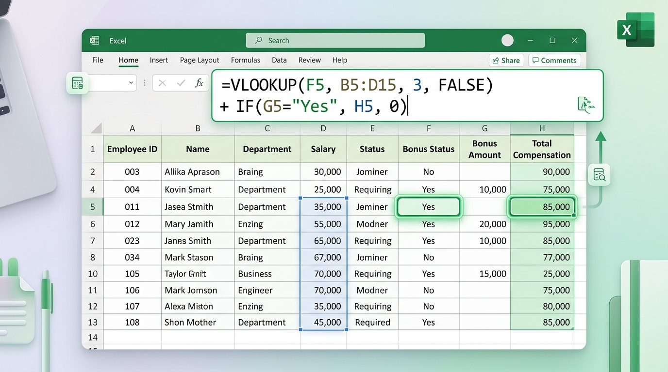
I remember a time when I was building an HR dashboard and forgot to add the FALSE argument. Excel couldn't find the exact employee ID and, instead of returning an error, it just brought back the salary of someone else with a "similar" ID. Imagine the nightmare that caused! So, engrave this in your mind: when in doubt, always end your VLOOKUP with a 0.
The Danger of Invisible Spaces (And How to Fix Them)
You look at cell A2 and you clearly see "12345". You look at the database on another sheet and you also see "12345". But VLOOKUP insists on throwing the dreaded #N/A error. What exactly is going on? Almost always, the answer is an invisible character: a trailing whitespace at the end of the text.
Corporate ERP systems and database exports love to add unnecessary spaces. To Excel, "12345" and "12345 " are completely different entities. If you are using Excel Online or Excel for Mac and you don't want to waste hours manually deleting spaces cell by cell, the solution is to wrap your lookup value inside the TRIM function.
=VLOOKUP(TRIM(A2),Sheet2!$A:$D,3,FALSE). Excel will magically remove all spaces before and after the text before executing the search. Goodbye, phantom #N/A errors!
Why VLOOKUP Breaks When You Insert a New Column
The Achilles heel of VLOOKUP is its reliance on hardcoded column index numbers. Let's say you wrote =VLOOKUP(A2,Customers!$A:$F,4,0) to fetch a customer's phone number, which happens to be in the 4th column. It works perfectly. But then, a colleague decides to insert a new column called "Date of Birth" right after the customer's name. What happens next?
The phone number column, which used to be the 4th, has now been pushed to become the 5th column. But your formula still has the number "4" hardcoded inside it. Result: your report is now displaying the Date of Birth where the phone number should be. To avoid this, advanced users in Excel 2021 often migrate to XLOOKUP, which doesn't suffer from this structural fragility. But if you have to use VLOOKUP for backward compatibility, there's a brilliant workaround.
You can use the MATCH function to automatically find the correct column number. It looks like this: =VLOOKUP(A2,Customers!$A:$F,MATCH("Phone",Customers!$A$1:$F$1,0),0). This way, if anyone adds, deletes, or moves columns, Excel recalculates the position of the "Phone" column entirely on its own. It's this level of dynamic automation that separates amateurs from Excel experts.
Locking Arrays: The Most Common Copy/Paste Error
You craft the perfect VLOOKUP on the very first row. You click, drag it down, and... everything from row ten downwards shows an error. What was the issue? You forgot to "lock" the table array, and the references slid down the sheet along with your formula.
When you don't use the dollar sign ($) for absolute references, the range A1:D100 becomes A2:D101, then A3:D102, and so on as you drag down. You end up losing the top rows of your data table. The fix is to select the array inside the formula bar and hit the F4 key on your keyboard. This instantly transforms A1:D100 into $A$1:$D$100.
Even better: instead of selecting a specific range of rows, you can select entire columns (e.g., $A:$D). Or, my personal favorite approach, turn your raw data into an official Excel Table (using Ctrl+T) and give it a name. Then, your VLOOKUP looks clean and unbreakable: =VLOOKUP(A2,CustomerTable,3,0). When you copy and paste, the name "CustomerTable" never shifts position.
Integrating VLOOKUP with IFERROR for Clean Dashboards
There is nothing uglier in a corporate report than dozens of cells screaming #N/A. When VLOOKUP doesn't find what it's looking for, it aggressively displays this error. In an executive dashboard or financial tracker, this gives off an impression of sloppiness or a broken file.
To fix this aesthetic nightmare in five seconds, wrap your VLOOKUP inside the IFERROR function. The logic is simple: "Excel, try to do the VLOOKUP. But if it errors out, write 'Not Found' or just leave it blank". The syntax is incredibly straightforward: =IFERROR(VLOOKUP(A2,Sheet2!$A:$D,3,0), "Not Registered").
If you prefer the cell to look completely clean and empty, just use two double quotes with nothing in between: =IFERROR(VLOOKUP(A2,Sheet2!$A:$D,3,0), ""). This small but vital aesthetic detail transforms an amateur spreadsheet into a professional, user-friendly system, saving you from explaining "just ignore those errors, it's normal" to your boss.
Frequently Asked Questions
1. Can VLOOKUP work with multiple criteria?
No, VLOOKUP won’t handle multiple criteria directly. You’ll need to combine values into a unique identifier or use an alternative approach like INDEX/MATCH for that.
2. What if my lookup value is in another worksheet?
Not a problem! You can reference another worksheet directly in your formula. Just make sure to include the sheet name followed by an exclamation mark. For example: =VLOOKUP(A1, 'Sheet2'!A1:B10, 2, FALSE).
3. Is VLOOKUP case-sensitive?
VLOOKUP is not case-sensitive. So, looking for "Laptop" will yield the same results as "laptop". If you need a case-sensitive lookup, you'll want to explore using INDEX/MATCH.
4. Can I use VLOOKUP with text data?
Absolutely! VLOOKUP works perfectly well with text data. Just be cautious about extra spaces or differences in capitalization that might affect your results.
5. What is the maximum number of rows VLOOKUP can handle?
The maximum number of rows depends on the Excel version and your system capabilities. Generally, Excel supports up to 1,048,576 rows, so you should have plenty of room!