
Understanding the SUMIF Function in Excel
If you've ever found yourself staring at a sea of numbers, trying to figure out how to sum up specific values based on certain criteria, you're not alone. The SUMIF function in Excel is an absolute lifesaver in such situations. Whether you're juggling monthly financial reports or checking the sales performance of various products, mastering this formula can save you a ton of time and headaches.
The beauty of SUMIF is its simplicity. It allows you to sum up values in a range based on a single condition. This can be particularly useful for tracking sales per product, expenses by category, or even tallying hours worked by employees in a specific department.
In Excel 365, for instance, you can easily navigate the interface with a few clicks to apply this function. Over the years, I’ve found that once you get the hang of SUMIF, it’s hard to imagine how you ever managed without it.
The Syntax of SUMIF
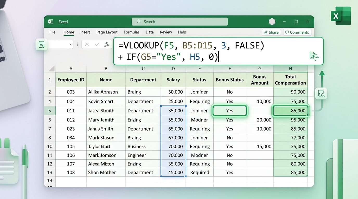
Before we dive into practical applications, let’s break down the syntax of the SUMIF function:
SYNTHAX: SUMIF(range, criteria, [sum_range])
- range: The range of cells you want to evaluate based on a specific condition.
- criteria: The condition that must be met for a cell to be included in the sum. This could be a number, expression, or cell reference.
- sum_range: (optional) The actual cells to sum. If omitted, Excel sums the cells in the range.
So, if you're trying to sum up sales for a specific product, your range might be the column listing products, while your sum_range would be the sales figures.
Practical Example: Summing Sales for Specific Products
Let’s say you have a sales report that tracks different products, their quantities sold, and total revenue. Your data might look something like this:
| Product | Quantity Sold | Total Revenue |
|---|---|---|
| Widget A | 120 | $1,200 |
| Widget B | 150 | $1,500 |
| Widget A | 80 | $800 |
| Widget C | 200 | $2,000 |
To sum up the total revenue for Widget A, your formula would look like this:
=SUMIF(A2:A5, "Widget A", C2:C5)
This tells Excel to look at the range A2:A5 for any occurrences of "Widget A" and then sum the corresponding values in C2:C5. Voila! You get the total sales revenue for Widget A, which amounts to $2,000 in this case.
Common Mistakes with SUMIF and How to Avoid Them
Now, here comes the fun part—common mistakes. I've seen it all, folks! One consistent error that users make is forgetting to ensure that the range and sum_range have the same number of rows. If they don’t match, Excel throws a tantrum and returns a #VALUE! error.
For instance, if your range is 10 rows and your sum_range is only 9, you’ll be left scratching your head wondering what went wrong. Always double-check your ranges!
Using Wildcards in SUMIF
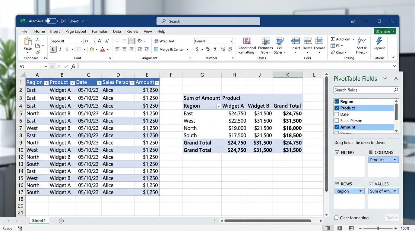
Did you know you could use wildcards in the SUMIF function? This is particularly handy if you're dealing with text criteria. For example, if you want to sum up all sales for products that start with "Widget," you can utilize the asterisk (*) wildcard to match any characters that follow. Here’s how you’d do it:
=SUMIF(A2:A5, "Widget*", C2:C5)
This formula sums up all revenues for products that start with "Widget," so you could capture any variations, like "Widget X" or "Widget Y." It’s super flexible and can save you loads of time when you're sifting through large datasets.
Dica DomineTec: When using wildcards, remember that they only work with text-based criteria, not with numbers!
Combining SUMIF with Other Functions
What if you want to take it a step further? You can combine SUMIF with other functions like IF, AVERAGE, or even VLOOKUP. For instance, imagine you want to calculate the average revenue per sale for Widget A. You can do this easily:
=AVERAGE(SUMIF(A2:A5, "Widget A", C2:C5)/SUMIF(A2:A5, "Widget A", B2:B5))
This formula first calculates the total revenue for Widget A and divides that by the total quantity sold for the same product, giving you the average revenue per sale. How’s that for maximizing your data analysis skills?
Real-World Applications of SUMIF
Let’s take a moment to appreciate the versatility of the SUMIF function in real-world scenarios:
- Financial Reporting: Quickly sum up various expense categories to understand where your money is going.
- Sales Tracking: Easily track sales figures by product, salesperson, or region.
- Inventory Management: Keep an eye on stock levels and understand which products are moving the fastest.
- HR Reports: Calculate total hours worked by department to streamline payroll processing.
In my experience, users often underestimate the power of this function. I once had a client who spent hours manually summing numbers in a gigantic spreadsheet. Once I showed them SUMIF, they were blown away by how much time they could save. Instant gratification, if you ask me!
Comparative Overview: SUMIF vs. SUMIFS
It’s easy to get SUMIF and SUMIFS mixed up, but they serve different purposes. Here’s a quick comparison to clarify:
| Function | Criteria | Syntax | Use Case |
|---|---|---|---|
| SUMIF | Single condition | SYNTHAX: SUMIF(range, criteria, [sum_range]) | Summing total revenues for one specific product |
| SUMIFS | Multiple conditions | SYNTHAX: SUMIFS(sum_range, criteria_range1, criteria1, [criteria_range2, criteria2], ...) | Summing total revenues for multiple products within a specific sales region |
So, the next time you’re contemplating which one to use, remember: if you’ve got multiple criteria to meet, SUMIFS will be your best friend.
FAQ Section
What Excel versions support the SUMIF function?
The SUMIF function is supported in all recent versions of Excel, including Excel 365, Excel 2021, Excel 2019, and Excel for Mac. No need to worry about compatibility issues here!
Can I use SUMIF with dates?
Absolutely! You can use the SUMIF function to sum values based on date criteria. Just make sure to format your dates correctly in Excel, and you can sum all sales that occurred after a certain date, for example.
What happens if there are no matching criteria?
If there are no matching criteria, the SUMIF function will return 0. It’s like that time you waited for an email response that never came—total radio silence!
Can I use SUMIF to sum based on text criteria?
Yes! The SUMIF function works perfectly with text criteria. Just be sure to enclose your text in double quotes, like "Sales" or "Complete".
What’s the maximum number of criteria I can use with SUMIFS?
With the SUMIFS function, you can use up to 127 different criteria. So, the sky's the limit when it comes to detailed filtering!
Wildcards: The Secret Sauce of SUMIF
Did you know that the SUMIF function is secretly a powerful text search engine? This is one of the most underrated features in Excel. Imagine you're dealing with an HR expense report, and the descriptions are a chaotic mess. You have entries like "Salary - John", "Advance Salary - Mary", and "Salary Ref. April". If you write a basic SUMIF looking exactly for the word "Salary", it will return zero because the cell contents aren't an exact match.
This is where wildcards save the day. The asterisk (*) represents any string of characters. By using the formula =SUMIF(A:A, "*Salary*", B:B), Excel will sum all amounts in column B where the word "Salary" appears anywhere inside the text in column A. There's also the question mark (?) wildcard, which substitutes for exactly one single character. For instance, searching for "A??" will sum rows matching "A01" and "A02", but ignore "A100". Mastering this simple shortcut eliminates the need for complex, nested string-manipulation formulas.
Dealing with Dates in SUMIF Conditions
A massive chunk of Excel work involves financial reporting, and financial reporting relies heavily on dates. A common rookie mistake is hardcoding the date directly into the criteria argument, like this: =SUMIF(A:A, "<12/31/2026", B:B). Sure, it works today, but next month, you'll have to manually hunt down and edit that formula. That is the opposite of an automated spreadsheet.
To build dynamic reports in Excel 365, Excel 2021, and earlier versions, you must learn to concatenate logical operators with volatile date functions. For example, to sum all overdue invoices (where the due date is before today), you should write: =SUMIF(A:A, "<" & TODAY(), B:B). Notice how the less-than sign is wrapped in quotes, and the ampersand (&) joins it to the TODAY() function. Whenever you open the workbook tomorrow, the criteria will update automatically. It's a game-changer for rolling dashboards and daily sales trackers.
SUMIF vs SUMIFS: When to Make the Switch
If you're just learning SUMIF, I need to share a slightly uncomfortable truth: in a professional corporate environment, you will almost always outgrow it. SUMIF is perfect for one-dimensional questions like, "What is the total revenue for the North region?" But in reality, your manager will ask, "What is the total revenue for the North region, for Product Y, during Q3?" The moment a second condition is introduced, your SUMIF breaks, and you must switch to SUMIFS.
The syntax order shifts when you make the jump. In SUMIF, the structure is =SUMIF(range, criteria, sum_range). In SUMIFS, the sum_range moves to the very front: =SUMIFS(sum_range, criteria_range1, criteria1, ...). Personally, I stopped using the basic SUMIF years ago. I use SUMIFS even if I only have a single condition. It builds good habits and ensures that if someone asks me to add a date filter next week, I don't have to rewrite the entire formula structure from scratch.
Why Your SUMIF is Returning Zero (And How to Fix It)
There is nothing more soul-crushing than carefully crafting a formula, pressing Enter, and seeing a giant, stubborn 0 looking back at you. Before you start questioning your life choices, check your raw data for invisible spaces. Corporate ERP systems (like SAP or Oracle) are notorious for exporting data with trailing spaces (e.g., "New York " instead of "New York"). SUMIF is extremely literal; it will not see those two strings as a match.
To quickly solve this without changing your source data, you can use the asterisk wildcard trick: =SUMIF(A:A, "New York*", B:B). Alternatively, create a helper column using the TRIM function to clean the text first. Another classic blunder is forgetting to lock your cell references. Always press F4 when highlighting your ranges (changing A1:A100 to $A$1:$A$100). If you don't anchor those ranges, dragging the formula down will cause the search area to slide down the sheet, leaving crucial data behind.
Leveraging Named Ranges for cleaner, error-free SUMIFs
Have you ever inherited a massive workbook from a colleague, only to be confronted with a formula that looks like this: =SUMIF('DataDump_Q4_Final'!$AC$5:$AC$1048576, "Approved", 'DataDump_Q4_Final'!$BR$5:$BR$1048576)? It takes immense brain power just to figure out what those columns represent. This is a classic symptom of poor spreadsheet architecture. If you want to build robust models, you need to start using Named Ranges in your formulas.
Instead of relying on rigid, ugly cell references, highlight your criteria column, click the Name Box (next to the formula bar), and type something logical like StatusList. Highlight your sum range and name it RevenueAmounts. Now, rewrite that beast of a formula: =SUMIF(StatusList, "Approved", RevenueAmounts). The difference is staggering. It reads like plain English. Not only does this practice make the spreadsheet instantly understandable to anyone who opens it, but it also completely removes the risk of forgetting to anchor your cells with F4. Combine this with official Excel Tables (Ctrl+T), and your named ranges will automatically expand when new data is pasted in, ensuring your dashboard is always 100% accurate without manual intervention.
A Note on Case Sensitivity
One critical limitation of the SUMIF function is that it is completely case-insensitive. If your data contains strings like "Apple" and "apple", the function will treat them as identical and sum their associated values together. For most financial or HR scenarios, this behavior is a blessing that forgives basic data entry typos. However, if you are working with strict identifiers—such as case-sensitive database IDs, server tokens, or specific passwords—SUMIF will fail you dramatically. To work around this and force a case-sensitive sum, you must abandon SUMIF entirely and use the SUMPRODUCT function combined with the EXACT function. This ensures Excel evaluates the exact capitalization before executing the math.