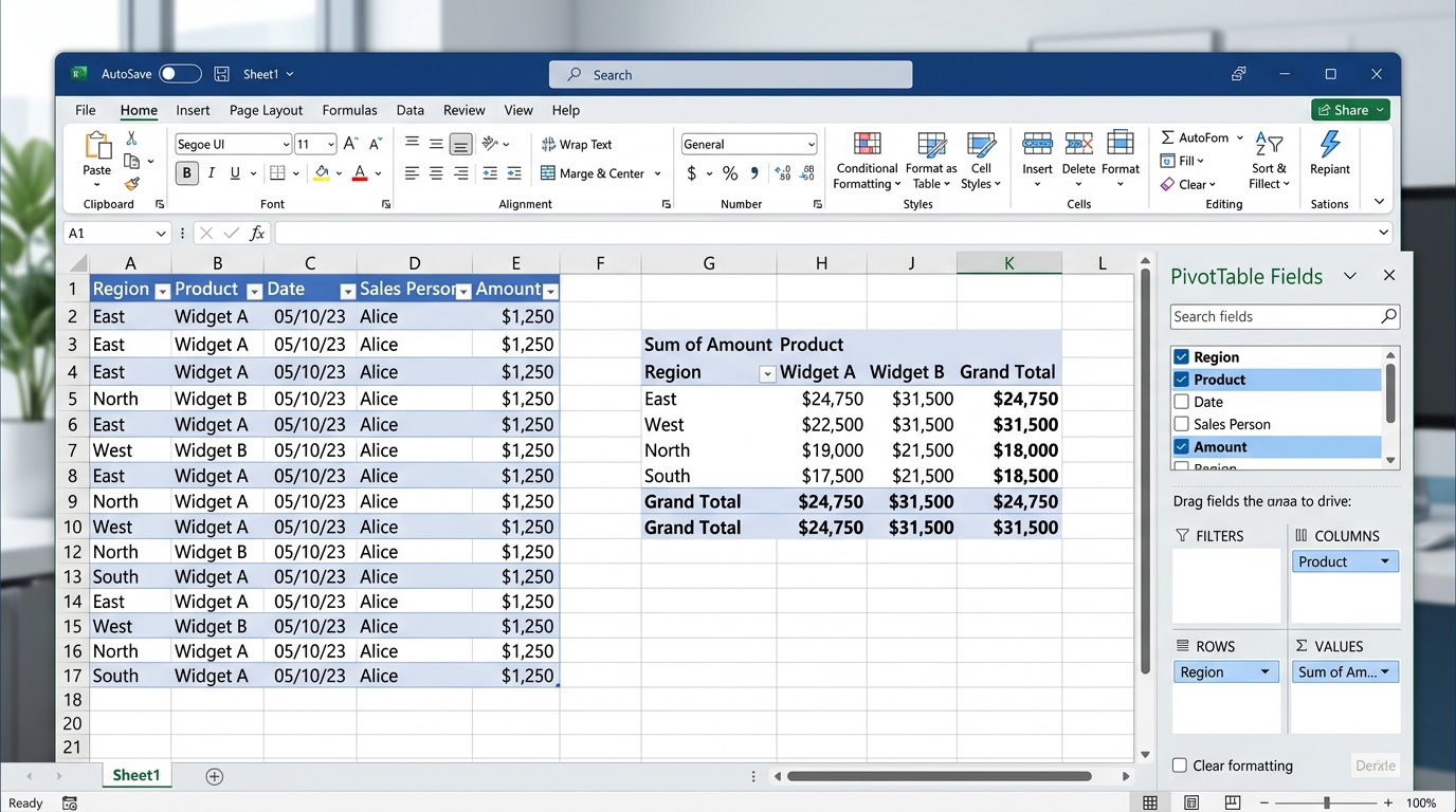
Understanding Freeze Panes in Excel
If you’ve ever been sifting through a lengthy Excel spreadsheet, you know the struggle of losing track of your headers after scrolling down a few rows. It's maddening! Luckily, Excel offers a feature called “Freeze Panes” that lets you lock specific rows or columns in place, so they remain visible no matter how far you scroll. This is especially useful for financial reports or tracking sales where you need to keep an eye on your headers.
Whether you're working with Excel 365, Excel 2021, or older versions like Excel 2019 or Excel for Mac, the process is pretty straightforward, and I’m here to walk you through it. Trust me, once you get the hang of it, you’ll wonder how you ever lived without this feature!
What's the Difference Between Freeze Panes, Split, and Unfreeze?
Before we get into the nitty-gritty of freezing panes, let's clarify some terms. In Excel, you have a couple of related features: Freeze Panes, Split, and Unfreeze. Understanding these will save you a ton of confusion!
- Freeze Panes: This locks specific rows or columns so they stay visible while you scroll.
- Split: This divides the window into two or four separate panes, allowing you to scroll independently within each section.
- Unfreeze Panes: This simply removes any freezing you’ve set up, allowing everything to scroll freely again.
In my experience, I use Freeze Panes much more frequently than Split because it provides a cleaner view. However, if you’re working with very large data sets that need detailed analysis, the Split function can be lifesaving.
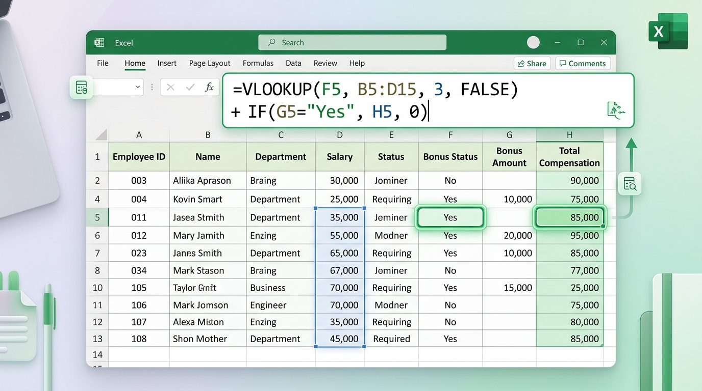
How to Freeze Panes in Excel
Now let’s get into the good stuff: how to freeze those pesky rows and columns! I'll break it down by version, but the steps are generally similar.
Step-by-Step Guide for Excel 365 and Excel 2021
- First, click on the cell below the row(s) you want to freeze and to the right of the column(s) you want to freeze. For instance, if you want to freeze Row 1 and Column A, click on cell B2.
- Next, navigate to the View tab on the Ribbon.
- Then, click on Freeze Panes in the Window group.
- Select Freeze Panes from the dropdown menu.
For Excel 2019 and Older Versions
The steps are pretty much identical. The only difference is that you might find the feature tucked away a bit differently. Look for the View tab, and you should still see the Freeze Panes option in the same spot.
Dica DomineTec: If you're using Excel for Mac, the process is the same, but make sure to check your keyboard shortcuts for added efficiency!
Freezing Multiple Rows or Columns
Need to freeze more than just the first row or column? No problem! Just select the cell that sits below the last row and to the right of the last column you want frozen. For instance, if you wish to freeze the first three rows and the first two columns, click on cell C4. Then follow the same steps as above.
Common Mistakes to Avoid
As with any feature, there are a few pitfalls to watch out for when using Freeze Panes. Here are some common mistakes I’ve seen, which you should try to avoid:
- Freezing the Wrong Rows or Columns: Always double-check which cell you’re selecting before you freeze. It’s easy to think you’re freezing the right thing, only to find out you’ve locked the wrong section.
- Forgetting to Unfreeze: If you start editing your spreadsheet and can’t see your changes because your panes are frozen, you’re not alone! Always remember to unfreeze when you don’t need the feature anymore.
- Not Saving Changes: Many users forget to save their workbook after making changes. If you don’t save, all your hard work goes down the drain!
Remember, practice makes perfect. The more you use this feature, the more intuitive it will become. Plus, your spreadsheets will look way more professional with clear headers that stay in view!
Practical Applications of Freeze Panes
So, when might you find yourself using Freeze Panes in real-world scenarios? Here are a couple of examples:
- Financial Reports: When analyzing quarterly revenue, freezing the header row with account names is invaluable. You want to see those names while scrolling through large datasets of numbers!
- Sales Tracking: If you're managing a sales team, you likely have key metrics at the top of your sheet. Freezing those rows keeps your KPIs front and center.
- Inventory Management: In any inventory spreadsheet, keeping track of product names and quantities while you navigate through long lists is essential. Freeze those top rows to make it easier!
In fact, I once managed a massive project where I had to compare data across multiple sheets. Freezing panes saved my sanity by keeping my categories visible at all times. Excel might sometimes feel like it’s out to get us, but features like this make the battle a little easier!
Unfreezing Panes
Now, if you find that you need to change what’s being frozen, unfreezing is just as simple. Here’s how:
- Go back to the View tab in the Ribbon.
- Click on Freeze Panes.
- Select Unfreeze Panes from the dropdown menu.
Remember, once you do this, it’s back to normal scrolling for all your rows and columns!
Exploring the Power of Excel 365 and Excel 2021
If you have ever found yourself staring at a massive financial dataset in Excel 365, you know how crucial the right tools can be. Many functions often live in the shadow of VLOOKUP, but their utility is unquestionable when dealing with reports where months or weeks are laid out in contiguous columns. Unlike older versions such as Excel 2019, recent releases bring an upgraded calculation engine that makes processing giant spreadsheets much faster, avoiding those dreaded crashes (we've all furiously hit Ctrl+S praying Excel doesn't close on us!).
The secret to mastering this is understanding how your data structure dictates performance. Imagine a retail sales dashboard: products are listed in rows, but the January-to-December results are spread across columns. Using the proper syntax allows you to instantly locate a specific month's revenue. By locking the array with the F4 key, you ensure that when you drag the formula down (or simply use Ctrl+C and Ctrl+V), the reference stays static, avoiding the classic #N/A error.
It is worth noting that while Excel Online is fantastic for collaboration, massive volumes of data searched via arrays might experience a slight delay during cloud recalculations. Still, for inventory management and dynamic HR dashboards, these functions remain a pillar of workplace productivity. And if you think you are limited to the basics, try combining features with the MATCH function to create dynamic row indices. This transforms a rigid spreadsheet into an intelligent query system worthy of a senior analyst.
Advanced Tips: Avoiding Common Errors and Optimizing Performance
Nobody likes opening a spreadsheet to find a sea of #N/A or #VALUE! errors. When this happens, panic might set in, but the solution is usually straightforward. One of the biggest culprits behind formula failures is invisible text formatting. You know that trailing whitespace that sneaks in when you export data from the company's ERP system? It prevents Excel from recognizing your search criteria. The golden tip here is to nest the TRIM function inside your formulas: =VLOOKUP(TRIM(A2), Array, 2, FALSE). This cleans the invisible garbage out of your data before the search even begins.
Another classic scenario happens in P&L (Profit and Loss) reports where new rows are constantly inserted. If you hardcoded the row index number in your formula (e.g., row 5), adding a new category above it means your spreadsheet will return the wrong value, as the desired row is now row 6. An elegant workaround is using the ROW() function combined, or better yet, formatting your data as a Table (shortcut Ctrl+T). Excel tables name ranges automatically, meaning your arrays dynamically scale with your data growth seamlessly.
Whether you are on Mac or Windows, the principle remains the same. In Excel for Mac, shortcuts like Command+C replace Ctrl+C, but the syntactical logic is entirely intact. I often joke that Excel is a universal language: once you grasp the fluency of arrays and absolute vs. relative referencing, the operating system is just a minor detail. Diving deep into the nuances of Excel is an investment that saves countless hours of manual, mind-numbing "copy and paste" work.
Integrating with Dashboard and Visualization Tools
When we start building visual dashboards, the accuracy of data extraction is paramount. This is where Excel joins forces with other tools to create flawless control panels. One of the smartest ways to deploy this logic is by tying it to dropdown menus (Data Validation). By allowing a user to select, say, the "Quarter" from a dropdown list, Excel works behind the scenes to fetch the exact column for that quarter and feed the primary chart.
Think about the daily grind of an HR department. Every month, they must compile overtime, time banks, and absences for dozens of employees. If the system generates horizontally oriented reports (days of the month across columns), it is the ideal conduit to extract specific info into an individual employee's file. If you make a mistake during the setup, a quick Ctrl+Z undoes the mess in a second, but a well-constructed layout greatly minimizes the need for manual intervention.
There is even more: when dealing with complex reports in Excel 365, you can also explore integrating your table with Power Query. Keep your data clean at the source, and use Excel simply as a display bridge. Remember, the secret to productivity isn't always using the most complex function out there; it is about using the right tool for the data structure you have. If your database grows horizontally (columns added over time), do not force a rigid layout. Accept the nature of your data and let the software do the heavy lifting for you.
Real-World Use Cases: Inventory and Sales Management
For those working in retail or e-commerce, inventory control can quickly become a logistical nightmare. Suppose you receive weekly price updates from suppliers, and these prices are delivered in spreadsheets where columns represent the weeks of the year. How do you efficiently update your cost base? The answer, once again, lies in the strategic use of native features.
By defining a robust structure, you can build a "Current Cost" table that always pulls the value from the latest registered week. This can be achieved by pairing lookups with functions that count non-empty cells (COUNTA). So, if you are currently in Week 42, the formula automatically locates that column and retrieves the product's value from the corresponding row. This level of automation eliminates manual typing, which is historically the primary cause of pricing errors.
Such practices are widely adopted by companies that demand agility in decision-making. I have seen many chaotic operational processes brought to order simply by introducing a solid reporting structure. The sheer flexibility of Excel 2021 and Microsoft 365 to rapidly recalculate dynamic arrays means that even 50,000-row, 100-column spreadsheets can run without lag—provided you avoid referencing entire infinite columns unnecessarily. Keep your data confined to the actual data boundaries to ensure top-tier performance.
Exploring the Power of Excel 365 and Excel 2021
If you have ever found yourself staring at a massive financial dataset in Excel 365, you know how crucial the right tools can be. Many functions often live in the shadow of VLOOKUP, but their utility is unquestionable when dealing with reports where months or weeks are laid out in contiguous columns. Unlike older versions such as Excel 2019, recent releases bring an upgraded calculation engine that makes processing giant spreadsheets much faster, avoiding those dreaded crashes (we've all furiously hit Ctrl+S praying Excel doesn't close on us!).
The secret to mastering this is understanding how your data structure dictates performance. Imagine a retail sales dashboard: products are listed in rows, but the January-to-December results are spread across columns. Using the proper syntax allows you to instantly locate a specific month's revenue. By locking the array with the F4 key, you ensure that when you drag the formula down (or simply use Ctrl+C and Ctrl+V), the reference stays static, avoiding the classic #N/A error.
It is worth noting that while Excel Online is fantastic for collaboration, massive volumes of data searched via arrays might experience a slight delay during cloud recalculations. Still, for inventory management and dynamic HR dashboards, these functions remain a pillar of workplace productivity. And if you think you are limited to the basics, try combining features with the MATCH function to create dynamic row indices. This transforms a rigid spreadsheet into an intelligent query system worthy of a senior analyst.
Advanced Tips: Avoiding Common Errors and Optimizing Performance
Nobody likes opening a spreadsheet to find a sea of #N/A or #VALUE! errors. When this happens, panic might set in, but the solution is usually straightforward. One of the biggest culprits behind formula failures is invisible text formatting. You know that trailing whitespace that sneaks in when you export data from the company's ERP system? It prevents Excel from recognizing your search criteria. The golden tip here is to nest the TRIM function inside your formulas: =VLOOKUP(TRIM(A2), Array, 2, FALSE). This cleans the invisible garbage out of your data before the search even begins.
Another classic scenario happens in P&L (Profit and Loss) reports where new rows are constantly inserted. If you hardcoded the row index number in your formula (e.g., row 5), adding a new category above it means your spreadsheet will return the wrong value, as the desired row is now row 6. An elegant workaround is using the ROW() function combined, or better yet, formatting your data as a Table (shortcut Ctrl+T). Excel tables name ranges automatically, meaning your arrays dynamically scale with your data growth seamlessly.
Whether you are on Mac or Windows, the principle remains the same. In Excel for Mac, shortcuts like Command+C replace Ctrl+C, but the syntactical logic is entirely intact. I often joke that Excel is a universal language: once you grasp the fluency of arrays and absolute vs. relative referencing, the operating system is just a minor detail. Diving deep into the nuances of Excel is an investment that saves countless hours of manual, mind-numbing "copy and paste" work.
Integrating with Dashboard and Visualization Tools
When we start building visual dashboards, the accuracy of data extraction is paramount. This is where Excel joins forces with other tools to create flawless control panels. One of the smartest ways to deploy this logic is by tying it to dropdown menus (Data Validation). By allowing a user to select, say, the "Quarter" from a dropdown list, Excel works behind the scenes to fetch the exact column for that quarter and feed the primary chart.
Think about the daily grind of an HR department. Every month, they must compile overtime, time banks, and absences for dozens of employees. If the system generates horizontally oriented reports (days of the month across columns), it is the ideal conduit to extract specific info into an individual employee's file. If you make a mistake during the setup, a quick Ctrl+Z undoes the mess in a second, but a well-constructed layout greatly minimizes the need for manual intervention.
There is even more: when dealing with complex reports in Excel 365, you can also explore integrating your table with Power Query. Keep your data clean at the source, and use Excel simply as a display bridge. Remember, the secret to productivity isn't always using the most complex function out there; it is about using the right tool for the data structure you have. If your database grows horizontally (columns added over time), do not force a rigid layout. Accept the nature of your data and let the software do the heavy lifting for you.
Real-World Use Cases: Inventory and Sales Management
For those working in retail or e-commerce, inventory control can quickly become a logistical nightmare. Suppose you receive weekly price updates from suppliers, and these prices are delivered in spreadsheets where columns represent the weeks of the year. How do you efficiently update your cost base? The answer, once again, lies in the strategic use of native features.
By defining a robust structure, you can build a "Current Cost" table that always pulls the value from the latest registered week. This can be achieved by pairing lookups with functions that count non-empty cells (COUNTA). So, if you are currently in Week 42, the formula automatically locates that column and retrieves the product's value from the corresponding row. This level of automation eliminates manual typing, which is historically the primary cause of pricing errors.
Such practices are widely adopted by companies that demand agility in decision-making. I have seen many chaotic operational processes brought to order simply by introducing a solid reporting structure. The sheer flexibility of Excel 2021 and Microsoft 365 to rapidly recalculate dynamic arrays means that even 50,000-row, 100-column spreadsheets can run without lag—provided you avoid referencing entire infinite columns unnecessarily. Keep your data confined to the actual data boundaries to ensure top-tier performance.
Frequently Asked Questions
1. Can I freeze both rows and columns at the same time?
Absolutely! Just select the cell that is below the rows you want to freeze and to the right of the columns you want to freeze, then follow the same freezing procedure.
2. What happens if I close and reopen my Excel file after freezing panes?
Your freezes will be saved, so you don’t need to set it up again unless you manually unfreeze it before closing the file.
3. Can I freeze more than one row or column?
Yes, you can freeze multiple rows or columns by selecting the appropriate cell as previously described. Just make sure to select the right cell before freezing!
4. Is there a limit to how many rows or columns I can freeze?
There’s no strict limit on how many rows or columns you can freeze, but practically, keeping it reasonable helps ensure you can still see your data effectively.
5. Will freezing panes affect printing my document?
No, freezing panes is a viewing feature. When you print, your document will show all rows and columns without any freezing applied.